
A gentle introduction to bootstrapping
In the previous post, I explained the general principles behind the standard error of the mean (or SEM). The idea underlying the SEM is that if you take repeated samples from the population of interest and take the standard deviation of the means of these samples, this gives you an estimate of the accuracy of the sample mean compared to the population mean. Formulas for the SEM are available for each distribution, and accurately reflect the degree of “fuzziness” in your sample mean if your data meet the assumptions of that distribution.
What if I’m not sure if my data meets the assumptions of a distribution?
You might have a case where the true population distribution of your sample doesn’t meet the assumptions of the closest appropriate distribution. For example, you might be interested in describing the mean levels of depression in a population, which is naturally positively skewed (i.e., most people in a population have no or low scores on measures of depression). In this case, using the SEM formula for the normal distribution would be inappropriate due to this skewness. Instead, you can create empirically derived SEMs using a technique called bootstrapping.
What is bootstrapping?
Bootstrapping involves basically the same principle as calculating the SEM I described in the last post, except instead of sampling from the population distribution, we resample from our sample distribution.
Let’s revisit the example from the previous post. We’ve been asked to calculate the mean number of page views a website receives per day. We decided to assess this by taking a sample of the daily number of page views over a 30-day period:
# Setting seed and generating a single sample
set.seed(567)
sample <- rpois(30, lambda = 220)
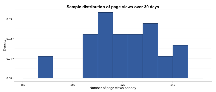
The mean of this sample is 219.6, which we will now treat as the population mean (without knowing the true population mean, we assume our sample mean is a very close approximation).
A Poisson distribution would be the most likely population distribution, as we are measuring a count of events over time. However, we’re not sure whether our sample of daily page views meets the assumptions of this distribution, and as such, we will bootstrap the SEM. To create a bootstrapped distribution of sample means, all we need to do is take repeated resamples from the distribution of our sample with replacement and take their means. The reason we must do this with replacement is because if we take a resample of 30 observations without replacement from our original sample, we will of course end up with the original sample for our resample!
An important thing to note is that because we are relying on the sample to describe the population distribution (instead of using a known distribution such as the Poisson), we have to make sure our sample is a good representation of our population. I will cover choosing a representative sample in next week’s blog post.
So let’s bootstrap our SEM in R. We will take our sample of 30 days of page views and take 1,000 resamples from this with replacement.
# Setting seed
set.seed(567)

# Generate the mean of each resample and store in a vector, and store each resample in a dataframe
mn_vector <- NULL
resample_frame <- data.frame(row.names = seq(from = 1, to = 30, by = 1))
for (i in 1 : 1000) {
    s <- sample(sample, 30, replace = TRUE)
    resample_frame <- cbind(resample_frame, s)
    mn_vector <- c(mn_vector, mean(s))
}

# Name the columns in the resample dataframe
names(resample_frame) <- paste0("n", seq(from = 1, to = 1000, by = 1))
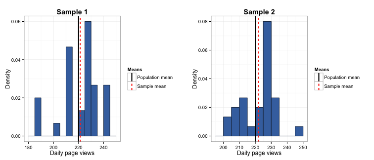
Because we resample with replacement, each resampling gives a slightly different estimate of the mean. For example, the mean in resample 1 is 221, and the mean from resample 2 is 222.
In the last blog post, I described how the mean of repeated samples from a population have a distribution that approximates the normal distribution. Similarly, the distribution of means of the resamples drawn from the sample also approximates the normal distribution.
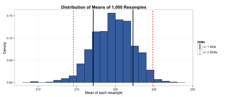
Taking the mean of this distribution of means gives us the population mean (219.7), and taking the standard deviation of this distribution gives us the SEM (2.6). Moreover, because this distribution of resample means is normal, we know that ±1 standard errors around the mean represents 68% of the means of the resamples, and ±2 standard errors represents 95% of the resamples. In other words, 68% of the time when we take a resample we will end up with a mean between 217.1 and 222.3, and 95% of the time when we take a resample we will end up with a mean between 214.7 and 224.7, a pretty small margin of error around our population mean of 219.6 page views per day.
How do I know if it is worth bootstrapping my SEM?
Let’s compare the result we get from just using the formula for calculating the SEM with the result we get from bootstrapping this sample. In the case of the Poisson distribution, this is \(\sqrt{\lambda / n}\).
# Defining lambda and n
lambda <- mean(sample)
n <- 30

# Calculating SEM
sem <- sqrt(lambda / n)
We get a result of 2.7, which is extremely close to our bootstrapped estimate (2.6). This is because the sample we took of daily page views met the assumptions of the Poisson distribution (given that it was drawn directly from it). In this case, bootstrapping our SEM does not improve our estimate of the SEM, therefore is not worth computing over simply using the SEM formula.
However, what if our population distribution did not fit a Poisson (or other) distribution? To demonstrate this, I have created a sample of 30 days of page views that is drawn from both the Poisson and uniform distributions. (If you are familiar with R, you can see I’ve created a Franken-distribution…)
# Setting seed and drawing non-Poisson sample
set.seed(567)
sample_np <- c(rpois(10, lambda = 220), runif(20, min = 180, max = 245))

# Generate the mean of each resample and store in a vector
mn_vector_np <- NULL
for (i in 1 : 1000) {
    s <- sample(sample_np, 30, replace = TRUE)
    mn_vector_np <- c(mn_vector_np, mean(s))
}

# Generate bootstrapped SEM
b_sem <- sd(mn_vector_np)

# Generate formula-derived SEM
f_sem <- sqrt(mean(sample_np) / 30)
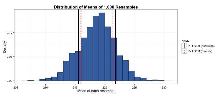
In this case, the SEM we obtain using bootstrapping is 3.1, compared to 2.7 using the formula. We can see that the formula-based SEM slightly underestimates the amount of fuzziness in our estimate of the sample mean (as demonstrated for ±1 SEMs below). In this case we would be better off using a bootstrapped SEM rather than calculating it using the formula for the Poisson distribution.
The take away message
Bootstrapping is a great technique to use when you are not sure if your data meet the assumptions of the closest appropriate distribution. This is a really common problem outside of the nice, clean world of simulations, and bootstrapping offers us to way to gain more accurate statistics from messy, real world data. While it may be a cumbersome method to use with very large data (as resampling from millions of observations is very time consuming), it can offer a convenient way of checking the robustness of your data to the assumptions of your distributions and gaining more accurate estimates in such situations.
Some of the points and code in this blog post are adapted from the excellent Statistical Inference unit on Coursera by Brian Caffo, Jeff Leek and Roger Peng.
Finally, the full code used to create the figures in this post is located in this gist on my Github page.