Interpreting linear regression coefficients

written October 28, 2015 in statistics, r, hypothesis testing, regression

Coming from a psychology background, I have a soft spot for multiple linear regression. This method is a workhorse in statistics and machine learning, being flexible, powerful and easily interpretable. An issue that people new to multiple regression face, however, is being overwhelmed by what all the coefficients represent and what the model is actually saying about the outcome variable. In this blog post I will show you that it is actually relatively straightforward to understand your regression model by talking you through how to interpret the coefficients of a model containing one continuous predictor, one factor predictor and their interaction in R.

Running the model

Let’s consider a model using the mtcars dataset. In this model, we will predict mpg (miles per gallon) using wt (the car’s weight in 1000lb increments), am (transmission type: automatic or manual) and their interaction term.

Before running the model, I will convert am into a factor variable. I could have also converted am to a factor within the model using factor(am), but I wanted to label each level to make the explanation of the coefficients more clear. Note that 0 = automatic and 1 = manual.

data(mtcars)
mtcars$am.f <- as.factor(mtcars$am); levels(mtcars$am.f) <- c("Automatic", "Manual")

# Build the model
model <- lm(mpg ~ wt + am.f + wt * am.f, data = mtcars)
summary(model)$coef

##                Estimate Std. Error   t value     Pr(>|t|)
## (Intercept)   31.416055  3.0201093 10.402291 4.001043e-11
## wt            -3.785908  0.7856478 -4.818836 4.551182e-05
## am.fManual    14.878423  4.2640422  3.489277 1.621034e-03
## wt:am.fManual -5.298360  1.4446993 -3.667449 1.017148e-03

Let’s start with the intercept

You can see from the output above that this model has four coefficients, the intercept, the main effect for wt , the main effect for am and the interaction of wt * am. So how do we interpret these? As you will recall, regression equations take the form:

$$ E[Y | X] = \beta_0 + \beta_1X $$

indicating that the expected value of $Y$, given the value of $X$, is calculated by adding the intercept to the value of $X$ multiplied by $\beta_1$. Our specific model is:

$$ E[Y | X_1X_2] = \beta_0 + \beta_1(weight) + \beta_2(transmission) + \beta_3(weight \cdot transmission) $$

Ok, so how do we interpret this? The first part is to understand that the intercept is the miles per gallon a car is expected to have when both car weight and car transmission are equal to 0. This can be seen when we substitute $X_1$ and $X_2$ for 0:

$$ \begin{aligned} E[Y | X_1X_2] &= \beta_0 + \beta_1(0) + \beta_2(0) + \beta_3(0 \cdot 0) \\ &= \beta_0 \end{aligned} $$

In this case the intercept, or the miles per gallon of an automatic car of weight 0 lbs, is 31.42. This intercept value is not very helpful as no real car can have a weight of 0. Therefore, before we go any further we need to make our coefficients more useful using a technique called centring.

Centring makes interpretation easier

Centring involves subtracting the mean from the continuous predictors in the model in order to change the point at which the regression slope crosses the intercept from 0 to the mean. This is demonstrated in the figure below:

plot of chunk centred_chart

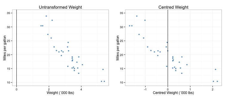
You can see that centring replaces the true intercept value for weight (0 lbs, a non-existent value) with a new intercept value (3.22) by making the model think of the mean as wt = 0. Let’s try and interpret our intercept again using our centred weight variable. Firstly, we need to run a new model:

centred.model <- lm(mpg ~ I(wt - mean(wt)) + am.f + I(wt - mean(wt)) * am.f, data = mtcars)
summary(centred.model)$coef

##                              Estimate Std. Error   t value     Pr(>|t|)
## (Intercept)                 19.235844  0.7356848 26.146856 3.243563e-21
## I(wt - mean(wt))            -3.785908  0.7856478 -4.818836 4.551182e-05
## am.fManual                  -2.167728  1.4188862 -1.527767 1.377893e-01
## I(wt - mean(wt)):am.fManual -5.298360  1.4446993 -3.667449 1.017148e-03

So, the new intercept value is 19.24, which is the predicted miles per gallon for an automatic car (transmission = 0) of weight 3217 lbs (centred weight = 0).

Now that we’ve covered the intercept, how do we interpret the rest? The trick is to break this down by the different levels of am. When the transmission is automatic (or when $X_2$ = 0), the regression equation becomes:

$$ \begin{aligned} E[Y | X_1X_2] &= \beta_0 + \beta_1(weight) + \beta_2(0) + \beta_3(weight \cdot 0) \\ &= \beta_0 + \beta_1(weight) \end{aligned} $$

Alternatively, when the transmission is manual (or when $X_2$ = 1), the regression equation becomes:

$$ \begin{aligned} E[Y | X_1X_2] &= \beta_0 + \beta_1(weight) + \beta_2(1) + \beta_3(weight \cdot 1) \\ &= \beta_0 + \beta_1(weight) + \beta_2 + \beta_3(weight) \\ &= (\beta_0 + \beta_2) + (\beta_1 + \beta_3)(weight) \end{aligned} $$

Substituting our model coefficients into this, we get:

$$ E[Y | X_1X_2] = 19.24 -3.79(weight) $$

for cars with automatic transmission and:

$$ \begin{aligned} E[Y | X_1X_2] &= (19.24 -2.17) + (-3.79 -5.3)(weight) \\ &= 17.07 -9.08(weight) \end{aligned} $$

for cars with manual transmission. So if we take a car that weighs 2620 lbs (which would have a value of -0.6 in our centred weight variable), our model predicts that it would have an MPG of 21.5 if it was automatic and 22.49 if it were manual.

When comparing the two models, you may have noticed that the two equations differ in both their intercept and slope values. More specifically, $\beta_2$ represents the change in the intercept when changing from automatic to manual transmission, while $\beta_3$ represents the change in slope changing from automatic to manual transmission. In other words, at the mean car weight, manual cars get 2.17 less miles per gallon than automatic cars. In addition, manual cars get 5.3 less miles per gallon for every additional 1000 lbs in weight. You can see this in the figure below. Note that the converse is true, and that manual cars gain 5.3 miles per gallon for every 1000 lbs less of car weight. As the slopes for the transmission types cross, at lower weights manual cars actually have better MPG than automatic cars.

plot of chunk interaction_model

Standard error and the confidence interval

The final part of interpreting regression coefficients is getting an estimate of their precision, which we will do using confidence intervals. We can shortcut the process of calculating these using R’s inbuilt predict function. The first step is create separate models for the automatic and manual transmissions.

centred.model.auto <- lm(mpg ~ I(wt - mean(mtcars$wt)), data = mtcars[mtcars$am == 0, ])
centred.model.manual <- lm(mpg ~ I(wt - mean(mtcars$wt)), data = mtcars[mtcars$am == 1, ])

We’ll then construct new dataframes containing the values of weight we want to put a confidence interval around. Let’s again go with 2620 lbs, which incidently corresponds to a manual car in our dataset, the Mazda RX4, and 3570 lbs, which corresponds with the Duster 360, an automatic car in our dataset. I’ve picked a 95% confidence interval (which is also the default in the predict function).

manual.car <- data.frame(wt = 2.620)
auto.car <- data.frame(wt = 3.570)

# CI for mean
manual.ci <- predict(centred.model.manual, newdata = manual.car, 
                     interval = ("confidence"), level = 0.95)
auto.ci <- predict(centred.model.auto, newdata = auto.car, 
                   interval = ("confidence"), level = 0.95)

For the manual car (the Mazda RX4), we can see that the predicted MPG is 22.49 and the 95% confidence interval is [20.76, 24.23]. The actual MPG of this car model is 21, which is within the confidence interval. Similarly, the predicted MPG for the automatic car (the Duster 360) is 17.9 and the 95% confidence interval is [16.64, 19.17]. However, the actual MPG for this model was 14.3, outside of the confidence interval, suggesting this is value for which the model is not a good fit.

A final note: using the model on existing versus new values

You can see above that when I used the model to predict MPG, it was only on values that were measured in the data. This is because when we want to use regression models to predict on new values, we have to use prediction intervals rather than confidence intervals. Prediction intervals are more conservative (wider) than confidence intervals to allow for the extra error that comes from using a value we haven’t measured. Prediction intervals are constructed using the same method as the confidence intervals above, but instead we pass “prediction” to the interval argument. Let’s say we want to predict the MPG for a car weighing 2000 lbs. Depending on whether the car is manual or automatic, the predicted value and prediction interval will be different, so we need to run it for both.

new.cars <- data.frame(wt = 2)

# Prediction interval for new values
manual.predict.ci <- predict(centred.model.manual, newdata = new.cars, 
                             interval = ("prediction"), level = 0.95)
auto.predict.ci <- predict(centred.model.auto, newdata = new.cars, 
                           interval = ("prediction"), level = 0.95)

You can see the predicted MPG for the 2000 lb manual car is 28.13 [95% prediction interval: 21.89, 34.36], and 23.84 [95% prediction interval: 17.67, 30.02] for the automatic car. You can also see that these intervals are significantly wider than the confidence interval.

A final note about both prediction and confidence intervals - they both become wider the further the value of interest is from the mean. This means that predicting outside of the range of measured values - always something that should be done with caution - will yield very wide prediction intervals compared to values within the observed range and close to the mean.

Much of the points and code in this blog post are adapted from the excellent Regression Models unit on Coursera by Brian Caffo, Jeff Leek and Roger Peng. This course gives a far more comprehensive coverage of this material and is highly recommended.

Finally, the full code used to create the figures in this post is located in this gist on my Github page.