
Two-group hypothesis testing: permutation tests
In the last blog post I described how you could test whether the difference between two groups was statistically significant using an independent-samples t-test. (I will rely heavily on that blog post in this one, so I encourage you to at least skim it before reading this.) I used the example that your company (a retail website selling children’s toys) had launched two advertising campaigns and wanted to see whether they brought in different amounts of revenue. I cheekily assumed that the population distribution of amount spent per site visit was approximately normally distributed. However, this is unlikely to be the case - you are much more likely to have a large number of visitors that buy nothing, a smaller number spending a small to moderate amount, and then a minority of visitors spending a lot.
What if my distributions are not normal?

(Image via Research Wahlberg)
In cases like this, we can’t use a t-test, so what can we do? We can instead rely on non-parametric methods. I will talk about one example, permutation tests, in this blog post. So how do they work? Well, when we collect our data (amount of money spent per visit), we assign it to a group depending on what advertising campaign the visit originated from. We then take the difference in the mean amount generated per campaign as our test statistic. What permutation tests suggest as their null hypothesis is that randomly reassigning (or permuting) these group labels and then taking the mean difference between these new groups will give a mean difference similar to the one we got from our original groups. In other words, the null hypothesis is that the group labels are arbitrary, and that we could get a mean difference of that size or bigger by chance alone. The alternative hypothesis is that the group labels are not arbitrary, and a mean difference of that size didn’t occur by chance. In permutation tests, we therefore permute the group labels a large number of times, and see where our original mean difference ranks among the permuted mean differences. This is a bit confusing, but I’ll talk you through it step-by-step.
Simulating some data
As with the last post, let’s say we collected a sample of 40 site visits for each campaign. To simulate the samples, I will resort to my much-loved method of creating Franken-distributions - in this case, I am merging elements of exponential and uniform distributions, plus throwing in some zero counts. This will give us some inflation around zero and a tapering off as the amount spent per visit increases, which is a far more realistic representation of the sort of data we’d collect.
data <- data.frame(group = rep(c("Campaign 1", "Campaign 2"), c(40, 40)),
                   amount.purchased = numeric(length = 80))

set.seed(567)
data$amount.purchased[data$group == "Campaign 1"] <- c(rep.int(0, 7),
                                                  rexp(33, rate = 1) * 100)
data$amount.purchased[data$group == "Campaign 2"] <- c(rep.int(0, 10),
                                                  rexp(30, rate = 2.5) * 100)
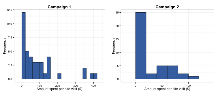
As you can see in the histograms below, the distribution of observations for campaign 1 appears to differ from that for campaign 2, so the group labels are not likely to be arbitrary. The frequency of observations where nothing or very little was spent in a visit is lower in campaign 1, and the maximum amount spent in any visit was higher.
Creating the test statistic
The next step is creating the test statistic to assess whether the difference between the campaigns’ revenue is meaningfully different. This is simpler than in the last post - we can use the raw mean difference rather than standardising it.
diff.means <- mean(data$amount.purchased[data$group == "Campaign 1"]) -
              mean(data$amount.purchased[data$group == "Campaign 2"])
The test statistic is 64.92, which indicates that visitors spent \$64.92 more per visit if they came to the site via campaign 1.
Permuting the group labels
We’ll now move on to the permutations. To illustrate how this works, I’ll start with a single example.
# Create a function that randomly reassigns each observation to a different group and then takes the mean difference between these new groups.
one.test <- function(grouping, variable) {
                resampled.group <- sample(grouping)
                mean(variable[resampled.group == "Campaign 2"]) -
                mean(variable[resampled.group == "Campaign 1"])
            }

# Example of how resampling works:
set.seed(567)
data$resampled.group <- sample(data$group)
rs.mean <- mean(data$amount.purchased[data$resampled.group == "Campaign 2"]) -
           mean(data$amount.purchased[data$resampled.group == "Campaign 1"])
head(data[ , c("group", "resampled.group", "amount.purchased")])
##        group resampled.group amount.purchased
## 1 Campaign 1      Campaign 2                0
## 2 Campaign 1      Campaign 2                0
## 3 Campaign 1      Campaign 2                0
## 4 Campaign 1      Campaign 1                0
## 5 Campaign 1      Campaign 1                0
## 6 Campaign 1      Campaign 1                0
What we’ve done here is randomly reassigned the group labels and taken the mean difference of the amount purchased per visit of these new groups. You can see this by comparing the ‘group’ and ‘resampled.group’ columns in the table above. The mean difference of this particular permutation is 11.2, compared to our test statistic of 64.92. We’ll now repeat this permutation process 1,000 times to get a distribution of the mean difference of the permuted groups.
perm.means <- replicate(1000, one.test(data$group, data$amount.purchased))
Rejecting or accepting the null hypothesis
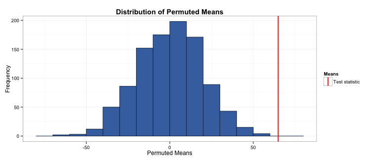
To check whether your test statistic is statistically different from 0, we just check how it ranks compared to the permuted means:
sig <- sum(perm.means > diff.means)
The number of permuted mean differences that exceeded the true mean difference was 0. As there were 1,000 permutations, the significance level is simply 1/1001, or p = 0.001. As this is less than 0.05, this means that campaign 1 generates significantly more income than campaign 2 per site visit.
Take away message
This is a brief introduction to permutation tests, which is a family that includes well-known non-parametric methods such as the Fisher’s exact and Wilcoxon rank-sum tests. These tests are a useful part of your statistical arsenal when your data don’t fit the assumptions of parametric tests (as is often the case). However, these of course aren’t a magical fix-all to your problems and must be used sensibly! As an example, a problem we might have could be that taking the mean of such skewed data is not particularly meaningful, therefore doing a test of mean differences does not make sense.
As part of writing this post, I heavily borrowed from the code used in Thomas Lumley and Ken Rices’ presentation for the Summer Institute in Statistical Genetics, and used code and explanations from Charlie Geyer’s tutorial from his class at University of Minnesota, Twin Cities.
Finally, the full code used to create the figures in this post is located in this gist on my Github page.