Planning your New Year’s Eve in Melbourne using data
Like I’ve said in a previous post I’m not a huge fan of crowds, so I tend to spend my New Year’s Eve at home. That’s totally as fun as going out, right?

For those of you with the patience to make your way into the city, I’ve put together a New Year’s Eve edition of my analysis of the pedestrian traffic in Melbourne CBD. Hopefully this will help you avoid the worst of the crowds and have a fun and low-stress NYE.
Reading in and preparing the data
As with the last post, I will be using the City of Melbourne’s publicly available dataset tracking the number of pedestrians per hour for major CBD locations. The map showing the locations of the sensors in these data is here.
pedestrians <- read.csv(url("https://data.melbourne.vic.gov.au/api/views/b2ak-trbp/rows.csv"))
Extracting the New Year’s Eve data
The first thing we need to do is to narrow the data down to just New Year’s Eve. To begin, we convert the string variable Date_Time into a true datetime variable (in the POSIXct format).
pedestrians$date <- as.POSIXct(as.character(pedestrians$Date_Time),
                               format = "%d-%b-%Y %H:%M")
We then have a look at how many years of data we have.
head(pedestrians$date, 1); tail(pedestrians$date, 1)
## [1] "2009-05-01 AEST"
## [1] "2015-09-30 23:00:00 AEST"
The earliest New Year’s Eve we have is 2009, and the latest is last year’s (2014), giving us 6 years in total. I’ve decided to start my analysis at 6pm on New Year’s Eve and finish at 4am on New Year’s Day. Let’s extract it now:
p.subset <- with(pedestrians, pedestrians
                  [(date >= "2009-12-31 18:00:00" & date <= "2010-01-01 04:00:00") |
                   (date >= "2010-12-31 18:00:00" & date <= "2011-01-01 04:00:00") |
                   (date >= "2011-12-31 18:00:00" & date <= "2012-01-01 04:00:00") |
                   (date >= "2012-12-31 18:00:00" & date <= "2013-01-01 04:00:00") |
                   (date >= "2013-12-31 18:00:00" & date <= "2014-01-01 04:00:00") |
                   (date >= "2014-12-31 18:00:00" & date <= "2015-01-01 04:00:00"), ])
p.subset <- p.subset[complete.cases(p.subset), ]
Checking the number of sites per year
We now have a dataset with the number of pedestrians by sensor site, year and hour. We can get an overview of the number of sites we have data on for each hour by running a frequency table on date and feeding this into a data.frame.
dates <- as.data.frame(table(p.subset$date))
Looking at this table, the later years have substantially more sites than the earlier years (17-18 in 2009-2012, compared to 30-32 in 2013-2014). We’ll keep this in mind when looking at how our sensor sites perform.
Create year and hour variables
Finally, we’ll extract the year and hour information from the date variable and convert them into labelled factor variables.
library(lubridate); library(plyr)
p.subset$hour <- hour(p.subset$date)
p.subset$hour <- revalue(as.character(p.subset$hour),
                         c("18" = "0", "19" = "1", "20" = "2", "21" = "3",
                           "22" = "4", "23" = "5", "0" = "6", "1" = "7",
                           "2" = "8", "3" = "9", "4" = "10"))
p.subset$hour <- as.numeric(p.subset$hour)
p.subset$hour <- factor(p.subset$hour,
                        labels = c("6pm", "7pm", "8pm", "9pm", "10pm", "11pm",
                                   "12am", "1am", "2am", "3am", "4am"))

p.subset$year <- as.numeric(0)
p.subset$year[p.subset$date >= "2009-12-31 18:00:00"
              & p.subset$date <= "2010-01-01 04:00:00"] <- 1
p.subset$year[p.subset$date >= "2010-12-31 18:00:00"
              & p.subset$date <= "2011-01-01 04:00:00"] <- 2
p.subset$year[p.subset$date >= "2011-12-31 18:00:00"
              & p.subset$date <= "2012-01-01 04:00:00"] <- 3
p.subset$year[p.subset$date >= "2012-12-31 18:00:00"
              & p.subset$date <= "2013-01-01 04:00:00"] <- 4
p.subset$year[p.subset$date >= "2013-12-31 18:00:00"
              & p.subset$date <= "2014-01-01 04:00:00"] <- 5
p.subset$year[p.subset$date >= "2014-12-31 18:00:00"
              & p.subset$date <= "2015-01-01 04:00:00"] <- 6
p.subset$year <- factor(p.subset$year,
                        labels = c("2009", "2010", "2011", "2012", "2013", "2014"))
We’re now ready to start planning your New Year’s Eve in Melbourne City!
Watching the fireworks display
You might be planning to watch the midnight fireworks to welcome in 2016. This year the City of Melbourne has planned four sites for viewing the fireworks display, which will all have very similar live music and entertainment from 9pm to 1am. The sites are King’s Domain, Treasury Gardens, Flagstaff Gardens and Docklands, as shown on this nice little map from the City of Melbourne.
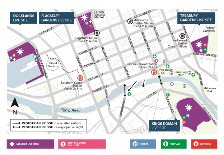
In order to have a look at the traffic associated with each of these sites, I found the closest sensors to each and marked them as belonging to the site in a new factor variable fireworks in the p.subset dataset.
As these fireworks events may not have been held in every year since 2009, I then checked whether the pattern of pedestrian traffic was the same for each year in the data. I did this by taking the mean number of pedestrians recorded by each sensor at the sites by each hour and year. I did this rather than taking the total number of pedestrians at each site as some of the sites have a much larger number of sensors than others, and as such, have an artificially inflated number of pedestrians. The mean number of pedestrians per sensors therefore serves as an average measure of density of pedestrians per site.
I’ve plotted each of the sites in separate graphs below.
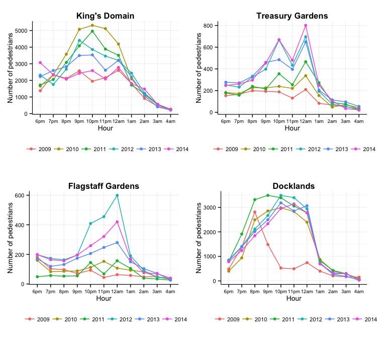
You can see that the pattern of traffic is not the same every year, especially for Treasury Gardens and Flagstaff Gardens. This is probably because either NYE activities at these sites has just started in the last couple of years, or they recently became more popular. Either way, it is probably more accurate to use the most recent year’s data (2014) to plot the potential traffic at the fireworks events this year, with a caveat that these patterns seem quite variable year-to-year in every site but Docklands.
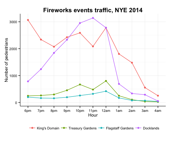
Despite the fact that the firework events being held at each of the sites look pretty much identical, Docklands and King’s Domain are far busier than Treasury Gardens and Flagstaff Gardens. It looks like your night will be far less crowded if you go to the celebrations at Flagstaff or Treasury Gardens. If you do want to go to one of the popular sites, you’d be better off going to Docklands and grabbing an early seat than trying to fight the crowds at King’s Domain.
Going out in the CBD
Instead of watching the fireworks, perhaps you are planning to go out in the CBD. To have a look at traffic in this area, I used the concentration of sensors around Elizabeth and Swanston Streets as this is where the majority of sensors in the city are located. I’ve separated them into 5 sites: Lonsdale Street, Chinatown, Bourke Street, Collins Street and City Square. I then categorised the corresponding sensors in the cbd variable in p.subset.
p.subset$cbd <- as.numeric(NA)
p.subset$cbd[p.subset$Sensor_Name %in%
                 c("Lonsdale St (South)", "Lonsdale Street (South)")] <- 1
p.subset$cbd[p.subset$Sensor_Name %in%
                 c("Chinatown-Swanston St (North)",
                   "Chinatown-Lt Bourke St (South)")] <- 2
p.subset$cbd[p.subset$Sensor_Name %in%
                 c("Bourke Street Mall (South)",
                   "Bourke Street Mall (North)",
                   "Bourke St-Russell St (West)",
                   "Bourke St-Russel St (West)")] <- 3
p.subset$cbd[p.subset$Sensor_Name %in%
                 c("Town Hall (West)", "Australia on Collins")] <- 4
p.subset$cbd[p.subset$Sensor_Name %in%
                 "City Square"] <- 5
p.subset$cbd <- factor(p.subset$cbd,
                        labels = c("Lonsdale Street", "Chinatown",
                                   "Bourke Street", "Collins Street",
                                   "City Square"))
Again, we’ll have a look at the mean number of pedestrians each sensor captures per hour, site and year.
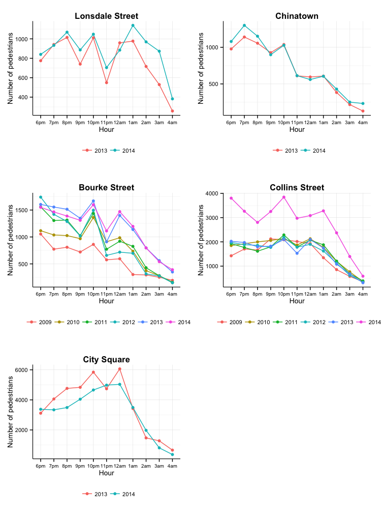
Three of the sites only have data for the last two years, suggesting that again using data from 2014 may be the best predictor of traffic in 2015.
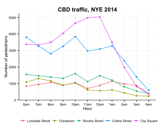
City Square is by far the busiest place in the CBD over the night, followed by Collins Street. It is much quieter around Bourke Street, Chinatown and Lonsdale Street. Even after 1am City Square and Collins Street are extremely crowded, so if you’re trying to get home you’d be better off trying the northern part of the CBD. Speaking of getting home…
Getting there and home
Ahhh, battling the crowds at the CBD events is one thing, but dealing with everyone at the train stations is another. To help you plan your journey in and out of the city, I’ve also looked at the city loop train station pedestrian traffic. As with my previous post, I have not included Parliament station as the sensors don’t really cover it properly. I’ve also included the traffic around the stations as part of the site as you’ll need to deal with these crowds to get in and out of the stations.
p.subset$stations <- as.numeric(NA)
p.subset$stations[p.subset$Sensor_Name %in%
                       c("Flinders St-Elizabeth St (East)",
                         "Flinders St-Swanston St (West)",
                         "Flinders Street Station Underpass")] <- 1
p.subset$stations[p.subset$Sensor_Name %in%
                       c("Southern Cross Station", "Spencer St-Collins St (North)",
                         "Spencer St-Collins St (South)")] <- 2
p.subset$stations[p.subset$Sensor_Name %in%
                       c("Melbourne Central", "State Library")] <- 3
p.subset$stations[p.subset$Sensor_Name %in%
                       c("Flagstaff Station")] <- 4
p.subset$stations <- factor(p.subset$stations,
                        labels = c("Flinders Street", "Southern Cross",
                                   "Melbourne Central", "Flagstaff"))
As with the other sites, I have taken the mean number of pedestrians per sensor, hour and year to get an indication of the density of pedestrians at each site.
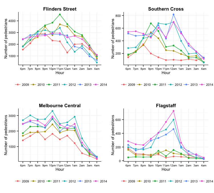
As with the other years, we see quite a bit of variance in traffic across the years, and we’ll therefore use the 2014 data to figure out the density of people at each of the stations across NYE.
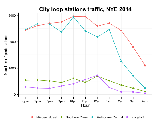
As we saw in the map I posted above from the City of Melbourne, Flagstaff and Melbourne Central will be closing at 11:45pm on New Year’s Eve. If you’re planning to go home before midnight, Southern Cross and Flagstaff are likely to be significantly less crowded than Flinders Street and Melbourne Central based on last year’s traffic. However, if you’re going to stay for the whole night you may be best trying to get to Southern Cross to avoid the crush at Flinders Street Station.
And with that, we’re done! Have a safe and fun New Year’s Eve, and I will see you in 2016!
