Doing hierarchical clustering with a precalculated dissimilarity index
Hierarchical clustering functionality in R is great, right? Between dist and vegdist it is possible to base your clustering on almost any method you want, from cosine to Canberra. However, what if you do want to use a different or custom method, and you’ve already calculated the distances separately? All of the documentation for the hclust function asks you to start with raw data from which R can calculate the distances between pairs. How do you get hclust to read in pre-calculated distance scores?
In this example, let’s say I’ve already manually calculated the Jaccard dissimilarity between each pair of cars from the mtcars dataset, and put them in a data.frame called carJaccard.
head(carJaccard)
##                car1      car2 jaccardDissimilarity
## 1         Mazda RX4 Mazda RX4          0.000000000
## 2     Mazda RX4 Wag Mazda RX4          0.002471232
## 3        Datsun 710 Mazda RX4          0.237474920
## 4    Hornet 4 Drive Mazda RX4          0.251866514
## 5 Hornet Sportabout Mazda RX4          0.461078746
## 6           Valiant Mazda RX4          0.211822414
So how do we get hclust to recognise this as a distance matrix? The first step is to reshape this data.frame into a regular matrix. We can do this using acast from the reshape2 package.
library(reshape2)
regularMatrix <- acast(carJaccard, car1 ~ car2, value.var = "jaccardDissimilarity")
We now need to convert this into a distance matrix. The first step is to make sure that we don’t have any NA’s in the matrix, which happens when you have pairings created in your matrix that don’t exist in your dataframe of dissimilarity scores. If there are any, these should be replaced with whatever value indicates complete dissimilarity for your chosen metric (in the case of Jaccard dissimilarity, this is 1).
regularMatrix[is.na(regularMatrix)] <- 1
We are now able to convert our matrix into a distance matrix like so:
distanceMatrix <- as.dist(regularMatrix)
Let’s throw it into hclust and see how we went!
clusters <- hclust(distanceMatrix, method = "ward.D2")
plot(clusters)

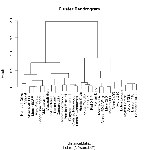
Great! As you can see from the dendogram above, we’ve ended up with what looks to be some fairly sensible looking clusters (well, at least to someone like me that knows nothing about cars - the ones with the same names are together so that looks good!).
We can also use the results of our clustering exercise to create groups based on a selected cutoff using the cutree function from the stats package. Looking at the dendrogram above, 0.5 looks like it will get us a good number of groups:
group <- cutree(clusters, h = 0.5)
(As an aside, you can also specify the number of groups you want using the k argument in cutree rather than the h, or height, argument. Check out help(cutree) for more details on this.)
The output of cutree looks … weird. Where are our groups? Never fear, we just need to take one final step in order to connect up our groupings with our car names.
groups <- as.data.frame(group)
groups$cars <- rownames(groups)
rownames(groups) <- NULL
groups <- groups[order(groups$group), ]
head(groups)
##    group          cars
## 1      1     Mazda RX4
## 2      1 Mazda RX4 Wag
## 3      1    Datsun 710
## 8      1     Merc 240D
## 9      1      Merc 230
## 10     1      Merc 280
As you can see, we just need to convert the results of cutree to a data.frame, which has the car names as the row names. In order to make it a bit neater, I’ve pulled the car names out into a column and ordered them based on the clusters.
As a final note, you may have noticed that I kept referring to dissimilarity scores in this post - this is for good reason! hclust is based on dissimilarity between pairs, rather than their similarity. I made this mistake the first time I used it and ended up with, to my puzzlement, a set of groups containing the most disparate pairs in the whole dataset! So learn from my foolishness and make sure you are using dissimilarity scores from the outset.
