Two-group hypothesis testing: independent samples t-tests

In some of my previous posts, I asked you to imagine that we work for a retail website that sells children’s toys. In the past, they’ve asked us to estimate the mean number of page views per day (see here and here for my posts discussing this problem). Now, they’ve launched two online advertising campaigns, and they want us to see if these campaigns are equally effective or one is better than the other (a technique known as A/B testing or randomised trials).

The way we assess this is a central method in statistical inference called hypothesis testing. The usual workflow of hypothesis testing is as follows:
1. Define your question;
2. Define your hypotheses;
3. Pick the most likely appropriate test distribution (t, Z, binomial, etc.);
4. Compute your test statistic;
5. Work out whether we reject the null hypothesis based whether your test statistic exceeds a critical value under this distribution.

This blog post will through each of these steps in detail, using our advertising campaign problem as an example.

Defining your question

The first, and most important step to any analysis is working out what you are asking and how you will measure it. A reasonable way to assess whether the advertising campaigns are equally effective or not could be to take all site visits that originate from each of the campaigns and see how much money the company makes from these visits (i.e., the amount of toys the customers who visit buy). A way we could then test if the amount generated differs is to take the mean amount of money made from each campaign and statistically test whether these means are different.

Defining your hypotheses

The next step is defining hypotheses so we can test these questions statistically. When you define hypotheses, you are trying to compare two possible outcomes. The first is the null hypothesis (\(H_0\)), which represents the “status quo” and is assumed to be correct until statistical evidence is presented that allows us to reject it. In this case, the null hypothesis is that there is no difference between the mean amount of income generated by each campaign. If we assign \(\mu_1\) to be the mean of the first population, and \(\mu_2\) to be the mean of the second population, these hypotheses can be stated as:

The alternative hypothesis (\(H_a\)) is that there is a difference between the mean level of income generated by each campaign. More formally, the alternative hypothesis is:

In other words, we are trying to test whether the difference in the mean levels of income generated by each campaign is sufficiently different from 0 to be meaningful.

Picking the most appropriate distribution

The most appropriate distribution for our test depends on what we assume the population distribution is. As the next step in our study of which campaign is correct, we take representative samples of site visits originating from each campaign and record how much was purchased (simulated below):

set.seed(567)
campaign.1 <- rt(40, 39) * 60 + 310
campaign.2 <- rt(40, 39) * 58 + 270

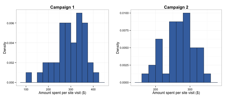
When we look at the data, it appears close enough to normal. However, our sample is a bit small (40 per campaign), so we should be a bit cautious about using the normal (Z) distribution. Instead, we’ll use a t-distribution, which performs better with “normally-shaped” data that have small sample sizes. According to our samples, the first advertising campaign generated a mean of \\(296.42 per visit with a standard deviation of \\)65.9, and the second campaign generated a mean of \\(267.11 per visit with a standard deviation of \\)43.53.

(Technical aside: The reason that the t-distribution performs better than the normal distribution with small samples is because we use the sample standard deviation in our calculation of both the t- and Z-distributions, rather than the true population standard deviation. At large samples, the sample standard deviation is expected to be a very close approximation to the population standard deviation; however, this is not the case in smaller samples. As such, using a Z-distribution for small samples leads to an underestimation of the standard error of the mean and consequently, confidence intervals. Incidently, this also means that as you collect more and more data, the t-distribution behaves more and more like the Z-distribution, meaning that it is a safe bet to use the t-distribution if you are not sure if your sample is big “enough”.)

Computing your test statistic

The next step is to get some measure of whether these values are different (the test statistic). When talking about hypothesis tests, I pointed out that the null hypothesis can be reframed as \(\mu_1 - \mu_2 = 0\), and the alternative hypothesis as \(\mu_1 - \mu_2 \neq 0\). As such, we can test our hypotheses by taking the difference of our two campaigns as the difference between the two means.

diff.means <- mean(campaign.1) - mean(campaign.2)

This gives us a difference between the campaigns of \\(29.31 per visit. In order to test whether this difference is statistically meaningful, we need to convert it into the same units as our test distribution (more on this below) by standardising it. To standardise the mean difference, we subtract the value of the mean difference under the null hypothesis (which is 0) from $\mu_1 - \mu_2\), and then divide it by the pooled standard error. This standardised mean difference is the t-value. (Of course, we don’t have the true population value of the means and standard deviations, so we use the sample estimates instead.)

# First calculate the pooled standard deviation (assuming equal variances, with equal sample sizes)
sp <- sqrt((sd(campaign.1)^2 + sd(campaign.2)^2)/2)

# Then calculate the standard error of the mean difference
se <- sp * (1 / length(campaign.1) + 1 / length(campaign.1))^.5

# The t-value is the difference in means divided by the standard error
t.value <- (diff.means - 0) / se

The t-value in this case is 2.347. We will work out if this is meaningful in the next step.

Rejecting or accepting the null hypothesis

The final step is working out whether our means are “different enough” is to define a rejection region around our mean of 0 (no difference). If our t-value falls within the rejection region, we can call our results statistically significant.

In order to define our rejection region, we need to first decide on our significance level. The significance level represents the probability of Type I error we are willing to tolerate in our study, or the probability that we reject the null hypothesis when it is actually true. The “benchmark” significance level is 0.05, or a 5% chance that we incorrectly reject the null hypothesis (in our case, saying the means are different when they are in fact not).

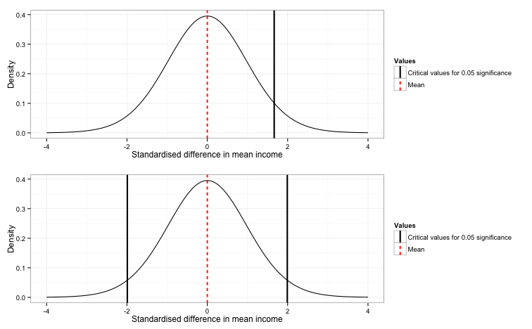
Once we have decided on our significance level, we need to find the critical values that represent the point beyond which 5% of our test distribution lies. The specific critical value depends on both the shape of the distribution and whether you are using a one-sided versus a two-sided test. One-sided tests are appropriate when you are trying to assess whether one value is bigger (i.e., \(\mu_1 - \mu_2 \gt 0\)) or smaller than another (i.e., \(\mu_1 - \mu_2 \lt 0\)). For example, if we were trying to test whether campaign 1 brought in more revenue than campaign 2, it would be appropriate for us to use a one-sided test. In this case, we would have the entire 5% rejection region in the right-hand tail of the distribution, as in the figure below.

However, as we are looking for any difference (whether positive or negative) between the two means, we must use a two sided test. In a two-sided test, the rejection region is split in half, so that 2.5% lies in the left-hand tail and 2.5% lies in the right-hand tail of the distribution. As you can see in the figure below, the implication of this is that we need less extreme test statistics to achieve significance in a one-sided test than in a two-sided, therefore it is very bad practice to incorrectly use a one-sided test when a two-sided test would be appropriate.

Just eat the damn orange!

Ok, after all of that, we can see whether our t-value lies in the rejection region. We generate the specific two-sided critical values for our distribution, and then compare this to our t-value.

# Generate the 95% confidence interval.
lci <- -1 * qt(c(.975), 78)
uci <- qt(c(.975), 78)

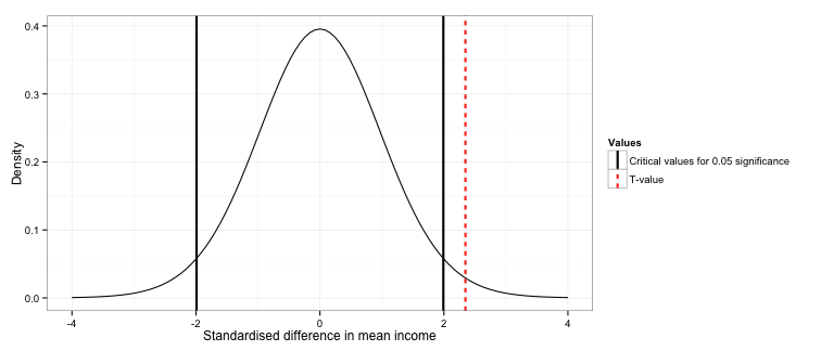
The rejection region lies below -1.991 and above 1.991. The t-value is 2.347, therefore we can say the difference in the outcomes generated between the two campaigns is significant at the 0.05 level.

Let’s repeat in R!

Now I’ve shown you how a t-test works under the hood, let’s go through how you would actually do this in your day-to-day use of R.

All we need to do is call the t.test function, like so:

test <- t.test(campaign.1, campaign.2, paired = FALSE, var.equal = TRUE)
test 

## 
##  Two Sample t-test
## 
## data:  campaign.1 and campaign.2
## t = 2.3473, df = 78, p-value = 0.02145
## alternative hypothesis: true difference in means is not equal to 0
## 95 percent confidence interval:
##   4.450556 54.169379
## sample estimates:
## mean of x mean of y 
##  296.4194  267.1094

As you can see, the results are the same. The t-value (or test statistic) is 2.347 and our p-value is 0.021, which is less than 0.05.

Statistical versus practical significance

In the end, we found out that the two advertising campaigns generated significantly different amounts of revenue per visit, with campaign 1 generating a mean of \$29.31 more per visit than campaign 2. However, does this automatically mean we go with campaign 1? For example, what if the reason that campaign 1 is generating more income is because the ads are being placed on high-end websites, where the sort of people seeing the ad have more disposible income than the general population, but the ad costs are much more expensive? Is the revenue difference big enough to justify the increased cost of advertising on this platform?

Take away message

In this post I talked you through a core technique in statistical inference, the two-sample t-test. While this is a very straightforward test to apply in R, choosing when it is an appropriate test to use and whether your data and hypotheses meet the assumptions of this test can be less clear. In addition, the results of a significant test must be interpreted in their practical context. I hope this has given you a starting point for analysing and interpreting the results of A/B testing and similar data.

Finally, the full code used to create the figures in this post is located in this gist on my Github page.