
Avoiding the crowds in Melbourne CBD using data
I love visiting the CBD of Melbourne - it is a beautiful place with great restaurants, cafes, shopping and museums. Unfortunately, as with any big city it can get really crowded at times, which can sap a bit of enjoyment for a nerd like me! Imagine my delight when I found that the City of Melbourne has a publicly available dataset of the number of pedestrians per hour for major CBD locations. The topic of this week’s blog post is therefore to help you to plan your journey around the city to avoid the crowds as best as possible.
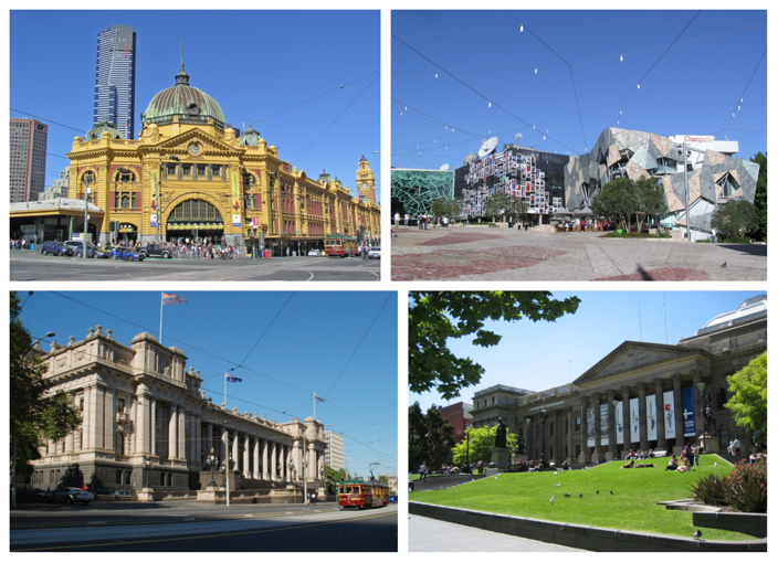
Some of the sights around Melbourne CBD (clockwise from top left): Flinders Street Station, Federation Square, the State Library of Victoria and Victorian Parliament House.
Reading in and preparing the data
The data were downloaded…
pedestrians <- read.csv(url("https://data.melbourne.vic.gov.au/api/views/b2ak-trbp/rows.csv"))
… and screened. None of the sensor sites had missing data.
head(pedestrians)
table(pedestrians$Sensor_Name)
tapply(pedestrians$Hourly_Counts, pedestrians$Sensor_Name, function(x) sum(is.na(x)))
Limiting the data to the last two years
In order to increase the relevance of the data to current pedestrian traffic, I limited the dataset to the final two years (from 1st October 2013 to 15th October 2015).
pedestrians$date <- as.POSIXct(as.character(pedestrians$Date_Time),
                               format = "%d-%b-%Y %H:%M")
p.subset <- subset(pedestrians, date >= "2013-10-01 00:00:00")
Discarding public holidays and public event days
To get the “normal” pedestrian traffic in the CBD, I removed all Victorian public holidays, as well as significant festivals and public events that might change how many people come into the city. These include New Year’s Eve and New Year’s Day, Australia Day, the White Night Festival, Labour Day/Moomba Festival parade, Easter long weekend, ANZAC day, Queen’s birthday, AFL Grand Final parade, Melbourne Cup, Christmas Day and Boxing Day.
p.subset <- with(p.subset, p.subset
                 [!(date >= "2013-11-05 00:00:00" & date <= "2013-11-05 23:00:00") &
                  !(date >= "2013-12-25 00:00:00" & date <= "2013-12-26 23:00:00") &
                  !(date >= "2013-12-31 00:00:00" & date <= "2014-01-01 23:00:00") &
                  !(date >= "2014-01-27 00:00:00" & date <= "2014-01-27 23:00:00") &
                  !(date >= "2014-02-22 00:00:00" & date <= "2014-02-23 23:00:00") &
                  !(date >= "2014-03-10 00:00:00" & date <= "2014-03-10 23:00:00") &
                  !(date >= "2014-04-18 00:00:00" & date <= "2014-04-21 23:00:00") &
                  !(date >= "2014-04-25 00:00:00" & date <= "2014-04-25 23:00:00") &
                  !(date >= "2014-06-09 00:00:00" & date <= "2014-06-09 23:00:00") &
                  !(date >= "2014-09-26 00:00:00" & date <= "2014-09-26 23:00:00") &
                  !(date >= "2014-11-04 00:00:00" & date <= "2014-11-04 23:00:00") &
                  !(date >= "2014-12-25 00:00:00" & date <= "2014-12-26 23:00:00") &
                  !(date >= "2014-12-31 00:00:00" & date <= "2015-01-01 23:00:00") &
                  !(date >= "2015-01-26 00:00:00" & date <= "2015-01-26 23:00:00") &
                  !(date >= "2015-02-21 00:00:00" & date <= "2015-02-22 23:00:00") &
                  !(date >= "2015-03-09 00:00:00" & date <= "2015-03-09 23:00:00") &
                  !(date >= "2015-04-03 00:00:00" & date <= "2015-04-06 23:00:00") &
                  !(date >= "2015-04-25 00:00:00" & date <= "2015-04-25 23:00:00") &
                  !(date >= "2015-06-08 00:00:00" & date <= "2015-06-08 23:00:00") &
                  !(date >= "2015-10-02 00:00:00" & date <= "2015-10-02 23:00:00"), ])
Reducing the number of sites
The map with all of the sensors is located here. To simplify things, I got rid of all of the sites outside of the CBD. In addition, I’ve collapsed some of the sensors that are close together into the same site (e.g., Bourke Street Mall (North) and Bourke Street Mall (South) became Bourke Street Mall). My definition of the city loop train stations includes sites that are close to the stations and are likely related to traffic for that station. For example, Flinders Street Station includes the sensors from the Flinders Street Station underpass, as well as those at the corners of Flinders Street/Elizabeth Street and Flinders Street/Swanston Street.
p.subset <- p.subset[!p.subset$Sensor_Name %in%
                         c("Australia on Collins", "Birrarung Marr",
                         "Lygon St (East)", "Lygon Street (West)",
                         "Grattan St-Swanston St (West)",
                         "Melbourne Convention Exhibition Centre",
                         "Monash Rd-Swanston St (West)", "New Quay",
                         "Sandridge Bridge", "St Kilda-Alexandra Gardens",
                         "The Arts Centre", "Tin Alley-Swanston St (West)",
                         "Victoria Point", "Waterfront City", "Webb Bridge"), ]

p.subset$Sensor_Name <- as.character(p.subset$Sensor_Name)
p.subset$collapsed_sensors <- p.subset$Sensor_Name
p.subset$collapsed_sensors[
    p.subset$Sensor_Name == "Bourke Street Mall (North)" |
    p.subset$Sensor_Name == "Bourke Street Mall (South)"] <- "Bourke Street Mall"
p.subset$collapsed_sensors[
    p.subset$Sensor_Name == "City Square" |
    p.subset$Sensor_Name == "Town Hall (West)"] <- "Swanston Street South"
p.subset$collapsed_sensors[
    p.subset$Sensor_Name == "Collins Place (North)" |
    p.subset$Sensor_Name == "Collins Place (South)"] <- "Collins Place"
p.subset$collapsed_sensors[
    p.subset$Sensor_Name == "Flinders St-Spark La" |
    p.subset$Sensor_Name == "Flinders St-Spring St (West)"] <- "Flinders St-Spring St"
p.subset$collapsed_sensors[
    p.subset$Sensor_Name == "Flinders St-Elizabeth St (East)" |
    p.subset$Sensor_Name == "Flinders St-Swanston St (West)" |
    p.subset$Sensor_Name == "Flinders Street Station Underpass"] <-
    "Flinders Street Station"
p.subset$collapsed_sensors[
    p.subset$Sensor_Name == "Southern Cross Station" |
    p.subset$Sensor_Name == "Spencer St-Collins St (North)" |
    p.subset$Sensor_Name == "Spencer St-Collins St (South)"] <- "Southern Cross Station"
p.subset$collapsed_sensors[
    p.subset$Sensor_Name == "Melbourne Central" |
    p.subset$Sensor_Name == "State Library"] <- "Melbourne Central"

p.subset$collapsed_sensors_2 <- p.subset$collapsed_sensors
p.subset$collapsed_sensors_2[
    p.subset$Sensor_Name == "Flinders St-Elizabeth St (East)" |
    p.subset$Sensor_Name == "Flinders St-Swanston St (West)"] <-
    "Flinders Street-Elizabeth/Swanston Sts"
p.subset$collapsed_sensors_2[
    p.subset$Sensor_Name == "Flinders Street Station Underpass"] <-
    "Flinders Street Station Underpass"
Averaging the pedestrian traffic
Finally, the number of pedestrians recorded was averaged over site, hour and weekday/weekend status.
# Sum the collapsed categories
library(plyr)
av_peds <- ddply(p.subset, c("date", "collapsed_sensors"), summarise,
                 n_peds = sum(Hourly_Counts))

# Extract weekday versus weekend
av_peds$day <- weekdays(av_peds$date, abbreviate = FALSE)
av_peds$weekend <- ifelse((av_peds$day == "Saturday" | av_peds$day == "Sunday"),
                           "Weekend", "Weekday")
av_peds$weekend <- as.factor(av_peds$weekend)

# Extract time of day
av_peds$time=format(as.POSIXct(av_peds$date, format="%Y-%m-%d %H:%M"), format="%H:%M")

# Collapse data to mean number of pedestrians per site, hour and weekend/weekday
av_peds <- ddply(av_peds, c("collapsed_sensors", "time", "weekend"), summarise,
                 mean_peds = mean(n_peds),
                 n_measurements = length(n_peds),
                 sum_peds = sum(n_peds))
City loop train stations

Four of the city loop train stations (see map above) were compared. The fifth station, Parliament, was not defined as only two sensors existed close to this station and therefore the number of pedestrians were likely to be underestimated. The average number of passengers per hour at each station was graphed, separated by weekend and weekday.
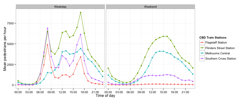
As you can see, Southern Cross and Flinders Street Stations (and surrounds) are the most congested in the morning on weekdays, while Melbourne Central has significantly less traffic. In the afternoons and evenings on weekdays, Flinders Street Station is by far the most busy station, while Flagstaff has the least traffic. On the weekends, Flinders Street Station has by far and away the most traffic, while Southern Cross is comparatively quiet (Flagstaff is so quiet as it is closed on the weekend).
station.hour <- ddply(stations, c("time", "weekend"), summarise,
                      total_peds = sum(sum_peds),
                      total_measurements = sum(n_measurements)
)
station.hour$av_peds <- station.hour$total_peds / station.hour$total_measurements
max.weekday <- station.hour$time[station.hour$av_peds ==
                                     max(station.hour$av_peds[
                                         station.hour$weekend == "Weekday"])]
max.weekend <- station.hour$time[station.hour$av_peds ==
                                     max(station.hour$av_peds[
                                         station.hour$weekend == "Weekend"])]
During the week, the stations are busy throughout the whole day, but the hour of peak traffic is 17:00, dropping off sharply before and after this time. You will therefore save yourself a transit headache by leaving the city a bit earlier or later. On the weekend, the stations become increasingly busy across the day, peaking at 15:00. From the looks of the graph above, your best bet on the weekends is to travel into the city in the morning and leave well before 15:00 to avoid the crowds.
The east of the CBD

The east side of the CBD is a lovely area, including Victorian Parliament House, two of the city’s theatres, high-end shopping and some wonderful restaurants (I recently went to Pastuso - it was incredible!). It tends to be quieter than other parts of the CBD, although it can get congested at times. Let’s have a look.
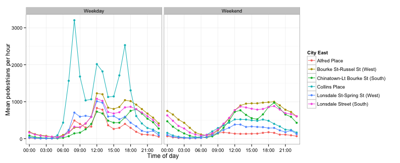
Collins Place is clearly the busiest on weekdays, especially at the start and end of the workday and at lunchtime. The rest of the east of the city has a similar pattern of pedestrian traffic during the weekday, becoming increasingly busier towards lunchtime, dropping off in the afternoon, and having another peak at the end of the workday/dinner time. The quietest areas appear to be Alfred Place and east Chinatown. On the weekends, the east of the CBD is quiet in the morning with increasing traffic towards the afternoon and evening. The busiest area is Bourke/Russell Streets, probably given its proximity to Her Majesty’s Theatre.
east.hour <- ddply(city.east, c("time", "weekend"), summarise,
                   total_peds = sum(sum_peds),
                   total_measurements = sum(n_measurements)
)
east.hour$av_peds <- east.hour$total_peds / east.hour$total_measurements
max.weekday <- east.hour$time[east.hour$av_peds ==
                                  max(east.hour$av_peds[
                                      east.hour$weekend == "Weekday"])]
max.weekend <- east.hour$time[east.hour$av_peds ==
                                  max(east.hour$av_peds[
                                      east.hour$weekend == "Weekend"])]
Unsurprisingly from the above graph, the peak time in the east CBD on weekdays is 12:00, suggesting an early or late lunch is prudent to avoid the crowds. Conversely, the peak time on weekends is 19:00, coinciding with the start of theatre shows and dinner time. Given that the crowds die down significantly after this, the best time to visit the east of the CBD on the weekend is either in the morning or after 19:00.
City centre

The centre of the city, running down Elizabeth and Swanston Streets, is by far the busiest part of the CBD. It includes some of the major shopping precincts of the city (Bourke Street Mall and Melbourne Central), as well as tourist attractions such as the Queen Vic Market, the State Library and Federation Square. In addition, there is a massive array of restaurants, bars and cafes (one of my favourite restaurants in this area is a Moroccan place called Sahara on Swanston Street).
In order to analyse the data for the city centre, I decided to separate out the sensors at the corners of Flinders Street/Elizabeth Street and Flinders Street/Swanston Street from the Flinders Street Station underpass and include them as a site in the CBD.
av_peds_2 <- ddply(p.subset, c("date", "collapsed_sensors_2"), summarise,
                 n_peds = sum(Hourly_Counts))

# Extract weekday versus weekend
av_peds_2$day <- weekdays(av_peds_2$date, abbreviate = FALSE)
av_peds_2$weekend <- ifelse((av_peds_2$day == "Saturday" | av_peds_2$day == "Sunday"),
                           "Weekend", "Weekday")
av_peds_2$weekend <- as.factor(av_peds_2$weekend)

# Extract time of day
av_peds_2$time=format(as.POSIXct(av_peds_2$date, format="%Y-%m-%d %H:%M"), format="%H:%M")

# Collapse data to mean number of pedestrians per site, hour and weekend/weekday
av_peds_2 <- ddply(av_peds_2, c("collapsed_sensors_2", "time", "weekend"), summarise,
                 mean_peds = mean(n_peds),
                 n_measurements = length(n_peds),
                 sum_peds = sum(n_peds)
)
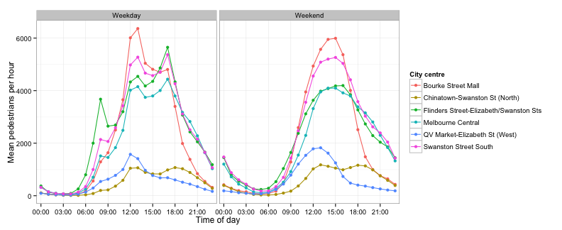
You can see straight away that the level of traffic in the CBD is substantially higher than in the east of the CBD, but is (naturally) comparable to the city loop train stations. Bourke Street Mall and Swanston Street South (Town Hall/City Square) are the busiest on both weekends and weekdays. In contrast, Chinatown and the Queen Vic Market are both much quieter than the other parts of the city. Melbourne Central and Flinders Street have much less traffic than Bourke Street Mall or Swanston Street South on the weekend, suggesting these might be better options for shopping or grabbing some food than other parts of the city centre.
centre.hour <- ddply(city.centre, c("time", "weekend"), summarise,
                     total_peds = sum(sum_peds),
                     total_measurements = sum(n_measurements)
)
centre.hour$av_peds <- centre.hour$total_peds / centre.hour$total_measurements
max.weekday <- centre.hour$time[centre.hour$av_peds ==
                                    max(centre.hour$av_peds[
                                        centre.hour$weekend == "Weekday"])]
max.weekend <- centre.hour$time[centre.hour$av_peds ==
                                    max(centre.hour$av_peds[
                                        centre.hour$weekend == "Weekend"])]
The busiest time on weekdays in the city centre is 13:00, suggesting that grabbing an early lunch might be a good strategy for avoiding the crowds. As with the train stations, traffic in the city centre increases across the course of the morning, peaking at 14:00, suggesting you are best coming into the city in the mornings.
The full code used to create the figures in this post is located in this gist on my Github page.