A crash course in reproducible research in R
A couple of weeks ago, I wrote a post giving you an introduction to reproducible research in Python. While the principles of reproducibility stay the same no matter the language you are using, there are some specific libraries and tools that R has that differ from Python. In this blog post, I’ll fill you in on how I conduct a reproducible analysis in R and, like with Python, you’ll see how straightforward it is!
Recap: What is reproducible research?
In the last post, I discussed that I think of an analysis as reproducible if you or another researcher can pick it up and continue to work on it with confidence that you fully understand the past work. In order for this to be possible, I think that you need to be able to answer 5 questions about your research:
1. What did I do?
2. Why did I do it?
3. How did I set up everything at the time of the analysis?
4. When did I make changes, and what were they?
5. Who needs to access it, and how can I get it to them?
As I explained in the last post, I use Git and Github (or insert your favourite version control and code-sharing tooling here) to track my changes and share my projects with collaborators, so we won’t revisit them in this post. However, R has some specific tools for points 1 to 3, so we’ll go over these in the rest of this post.
What did I do?
As I spoke about in the last post, one of the biggest issues you will face with remembering what you did in your analysis is if you do things manually. As with Python, R has some great functionality for downloading data from online sources and cleaning up those data once you’ve imported them.
It’s straightforward to access structured data from online sources and import them into R as data.frames. Below, I’ve created a function to download the .csv file containing the life expectancy data that I talked about in the last post. As you can see, you only need to use a couple of commands (the getURL and textConnection commands from the RCurl package). As well as being easy, it is completely reproducible!
install.packages("RCurl"); library(RCurl)

dataImport <- function(dataurl) {
  url <- dataurl
  dl <- getURL(dataurl, ssl.verifyhost=FALSE, ssl.verifypeer=FALSE)
  read.csv(textConnection(dl), header=T)
}

life <- dataImport("http://apps.who.int/gho/athena/data/xmart.csv?target=GHO/WHOSIS_000001,WHOSIS_000015&profile=crosstable&filter=COUNTRY:*&x-sideaxis=COUNTRY;YEAR&x-topaxis=GHO;SEX")
R also has great functionality for cleaning up datasets. Below, you can see I was able to create a short function using only commands from base R to select the appropriate subset of columns and rows in our newly imported dataset, as well as rename the remaining columns.
cleaningData <- function(data, startrow, columnyear, year, colsToKeep, columnNames) {
  df <- data[c(startrow:nrow(data)) & data[[columnyear]] == year, ]
  df <- df[ , colsToKeep]
  names(df) <- columnNames
  df
}

life <- cleaningData(life, 2, "X.1", " 2015", c("X", "X.1", "Life.expectancy.at.birth..years."),
                      c("Country", "Year", "LifeExpectancy"))
Why did I do it?
Like Python, R has its own tooling for literate statistical programming called R Markdown. Just like with Juypter notebooks, you can write chunks of markdown text alongside R code, meaning you can create easy-to-read, meaningful annotations for your analysis. You can also include results, tables and charts, allowing you to create reports and other documents from one self-contained R Markdown script. In fact, Mauricio and I wrote our book on graphing in ggplot2 entirely using R Markdown!
How do I set up an R Markdown document?
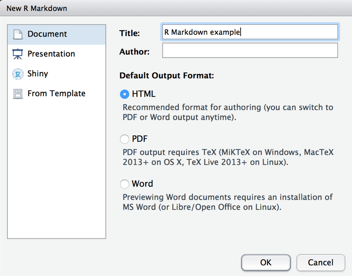
R Markdown documents can be created within RStudio (like much of the best R functionality!). To open a new R Markdown document, simply choose ‘R Markdown’ as the type when creating a new file. You’ll be asked to give your R Markdown document a title; I’ve called this one ‘R Markdown example’. Then click ‘OK’ to initialise the new document.

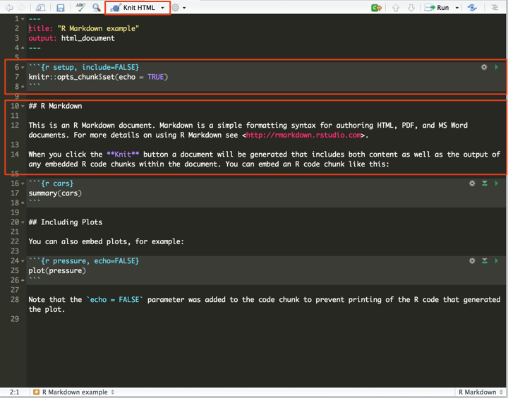
R Markdown documents automatically start with a template. As you can see, there are two types of code within an R Markdown document. Code is placed within chunks, which are delimited by backticks and {r}. There are many options available that allow you to customise how the code is presented and run within the chunks, but the default is that they will simply run whatever R code is inside them. Outside of the chunks, any text written is recognised as markdown. To run an R Markdown document, press the ‘Knit HTML’ button at the top of the document. This renders the markdown and executes the R code, and spits it out in an HTML document.

You can export R Markdown documents in a variety of formats, which you can control by using the knit function within the knitr package. To do this, we feed in our R Markdown file as the input, and specify the name of your rendered file and the desired format as the output. Here, I’m rendering our example document as a regular markdown file:
install.packages("knitr"); library(knitr)

knit("/Users/jodieburchell/Documents/r-reproducible/R Markdown example.Rmd",
     output = "/Users/jodieburchell/Documents/r-reproducible/R Markdown example.md")
And it’s really that simple! You can see how easily you can integrate literate statistical programming into your usual RStudio workflow.
How did I set it up?
Like with Python, your scripts in R can fail because you are using the wrong version of a library, or because two different libraries that you have installed globally don’t play nicely together. R has a similar solution to Python’s virtualenvs called packrat which allows you to keep track of your analyses’ dependencies.
Packrat is an R library that allows you to create a special kind of directory that works in a very similar manner to a virtualenv. While you are within the packrat directory, any libraries you install are isolated: these libraries are only available to your specific project, and your project cannot access any libraries installed outside of it. Packrat folders are able to keep track of your dependencies due to the presence of a lock file, which simply keeps track of what libraries you installed and their versions (much like the frozen requirements file in virtualenvs).
How do I set up a packrat file?
I’ll run through how to set up a packrat directory as part on an RStudio project, but there is also a great tutorial by RStudio on how to do so independent of a project.
The first step is to globally install packrat on your machine.
install.packages("packrat")
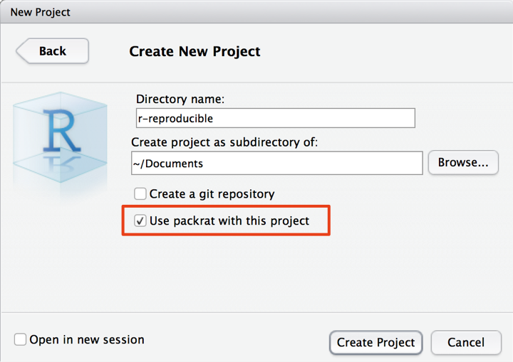
Once you’ve done that, restart RStudio. This should be the only time you need to do this. Once you’re back in RStudio, create a new RStudio project in a new directory (instructions on how to do this here). At this point, you’ll be asked to name your new project, and most importantly, indicate whether you want to make it a packrat project. As you can see below, it is as simple as ticking a box to initialise your packrat directory!

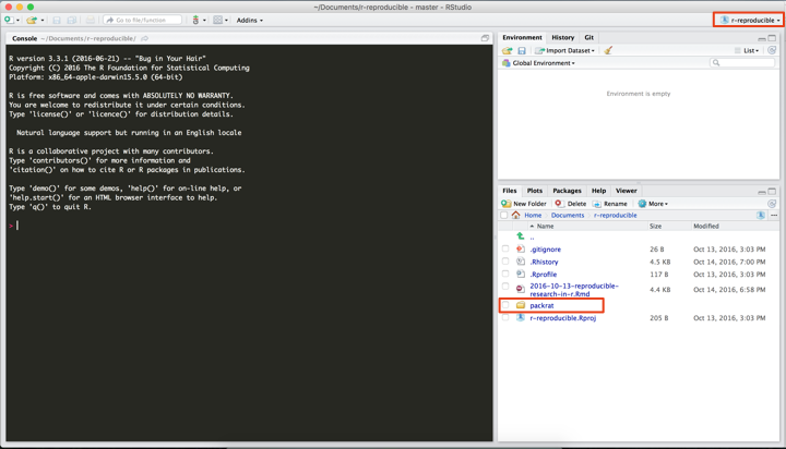
Once we’ve created our new RStudio project with packrat, you can see we have a new folder in our directory called ‘packrat’. Among other things, this is where your lock file lives that keeps track of all of the packages you install.

Installing libraries is super simple - while we are in our project we can use the regular install.packages command, and it will keep the installation limited to this specific project. Let’s install ggplot2.
install.packages("ggplot2"); library(ggplot2)
If you’re following along, you can see that even if you have ggplot2 system installed, R ignores this and does a clean installation. This is because it cannot access your globally-installed version of ggplot2 and needs to install it from scratch.
RStudio projects with packrat are set up with automatic snapshots, meaning that packrat keeps track of any changes you make to your project dependencies without you needing to explicitly snapshot them yourself.
Finally, sharing, or coming back to your own packrat project on a different machine is really easy. RStudio does pretty much all of the heavy lifting, so all you need to do is install the project directory on the new machine and open the project in RStudio. All of the project dependencies will be automatically installed, leaving you ready to pick up the project and go from where you left off.
In my mind, the simplest way to share your RStudio project directory is by pushing it to a remote repo on something like Github, and cloning it to your machine when you next need to work on it. As discussed in the previous post, this also has the additional advantage of allowing you to keep track of changes to your project.
I hope this tutorial has shown you how few changes you need to make to your usual analysis workflow in R in order to ensure your work is reproducible. Implementing these steps will mean you and others will be happily building on your projects for years to come!
