Exploring decision tree modelling with DataSpell
During my years of working as a data scientist, I’ve tried quite a number of IDEs. When I was primarily working with R, RStudio was a very nice environment to work with, but when I moved to working in Python I hadn’t been able to find anything close. Over the years, I’ve tried working with just notebooks, experimented with Spyder and Rodeo, and have settled on a combination of JupyterLab for my research workflow and PyCharm when I want to write code intended for production.
However, moving between two different IDEs creates a lot of friction when doing data science work, as it involves task switching and introduces needless distractions. This is particularly due to the fact that the flow of a data science project often iterates between the research and development phases. I was therefore very excited to hear that JetBrains has released a new IDE called DataSpell specifically designed to support data science work. This IDE aims to take those features from PyCharm that we all know and love, such as smart code completion and dependency management, while at the same time making notebooks first-class citizens. In addition, there are a number of other nice features that make doing a data science project that much nicer, which I’ll show in this blog post. I should note that DataSpell also supports R natively, but in this post I’ll be focusing on it’s capabilities with a Python project.
To explore what DataSpell can do, I’ll be creating a simple decision tree model using the Heart Failure Prediction DataSet, which was kindly uploaded to Kaggle by Federico Soriano Palacios. In this analysis, we’ll be reading in the data, doing some simple feature engineering, checking the model accuracy using cross-validation, and exploring a decision tree visualisation package called pybaobab which makes interpreting decision trees easier.
Accessing the data
Obviously, the first step is to access our data. I wanted to first show a really cool feature of DataSpell, which is its ability to support connections to databases. I really like DataGrip, so the introduction of some of the features of DataGrip into DataSpell is a very welcome addition for me.
For this project, I created a local PostgreSQL database in a Docker container. I then loaded my data into a table in this database using pandas, sqlalchemy and psycopg2. I will describe how I did this in another blog post, but for now, I want to show how easy it is to connect to this database within DataSpell and then view the table contents.
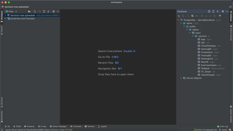
By clicking on the “Database” tab to the right of the IDE, and then clicking on “New”, I was able to easily create a connection to my database just by specifying the database name, user and password (JetBrains has instructions on how to connect to a range of databases here). As you see below, I am now easily able to view the contents and schema of my table.
Setting up the environment
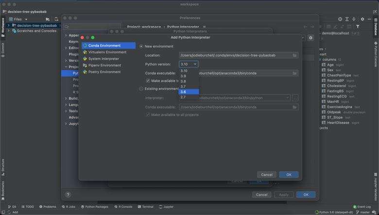
As said above, I will be using pybaobab to help me interpret my decision tree models. However, annoyingly, this package is only compatible with Python 3.6, which I no longer have installed globally on my machine.
Luckily, DataSpell offers the ability to set up your Python interpreter using a range of methods, including Conda. This means I was quickly and easily able set up a Python 3.6 virtual environment using Conda, as you can see below. Detailed instructions on how to do this are here.
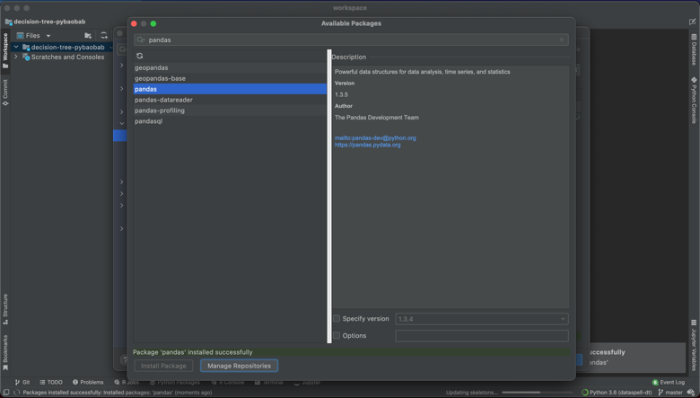
This project required sklearn, numpy, pygraphviz, matplotlib, and pandas. I was able to add all of these dependencies through the UI, as below.
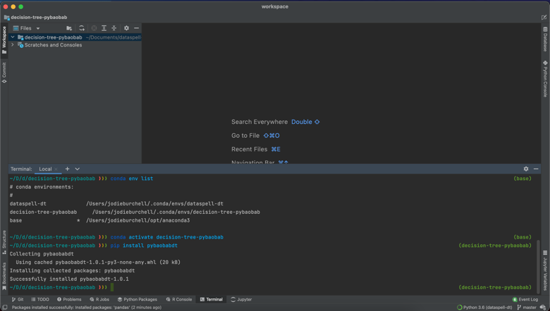
The only exception was pybaobabdt itself, which is only available through pip for the moment. However, the built in Terminal meant that I was easily able to activate my Conda environment and then pip install the missing package. You can also see that this also makes it possible to install your Conda packages using the command line.
Feature engineering and modeling with DataSpell notebooks
In order to get started in DataSpell, you simply attach a directory. I selected a location on my machine to save my project and was then able to get started by creating a new Jupyter notebook.
To get started, I first imported my dependencies and read in my data.
import pandas as pd
import numpy as np
import pybaobabdt

from sqlalchemy import create_engine

from sklearn.tree import DecisionTreeClassifier
from sklearn.model_selection import cross_val_score

engine = create_engine('postgresql://jodie:hello@localhost/demo')

heart = pd.read_sql("SELECT * FROM heart", engine)
I then checked each of the categorical features and the target.
for field in ["HeartDisease", "Sex", "ChestPainType", "RestingECG",
              "ExerciseAngina", "ST_Slope"]:
    print(f"\nData field: {field}")
    print(heart[field].value_counts())
Data field: HeartDisease
1    508
0    410
Name: HeartDisease, dtype: int64

Data field: Sex
M    725
F    193
Name: Sex, dtype: int64

Data field: ChestPainType
ASY    496
NAP    203
ATA    173
TA      46
Name: ChestPainType, dtype: int64

Data field: RestingECG
Normal    552
LVH       188
ST        178
Name: RestingECG, dtype: int64

Data field: ExerciseAngina
N    547
Y    371
Name: ExerciseAngina, dtype: int64

Data field: ST_Slope
Flat    460
Up      395
Down     63
Name: ST_Slope, dtype: int64
You can see that the target is quite balanced, which will make building the classifier easier. There are also have a number of categorical features which are string encoded, and in some cases, have more than one level. I’ll need to convert these to one-hot encoded features to be able to use them in the classifier. I’ll also convert the outcome to a labelled bytes column so that in the visualisation I will have clear labels for each split of the tree.
def generate_one_hot_encoding(data_field: str) -> pd.DataFrame:
    return pd.get_dummies(heart[data_field],
                          columns=heart[data_field].unique().tolist(),
                          prefix=data_field)

for feature in ["ChestPainType", "RestingECG", "ST_Slope"]:
    heart = heart.join(generate_one_hot_encoding(feature))

heart["SexBin"] = np.where(heart["Sex"] == "M", 1, 0)
heart["ExerciseAnginaBin"] = np.where(heart["ExerciseAngina"] == "Y", 1, 0)

heart["HeartDiseaseBytes"] = np.where(heart["HeartDisease"] == 1, "disease", "no_disease").astype("bytes")
Next, I’ll take all of the features and build a simple decision tree classifier. I’m not going to get fancy here as I’m just demoing a few things, so I’ve left in all of the features despite quite a few of them being highly imbalanced, and just used the default hyperparameter values.
y = list(heart["HeartDiseaseBytes"])
features = ['Age', 'RestingBP', 'Cholesterol', 'FastingBS',
            'MaxHR', 'Oldpeak', 'ChestPainType_ASY', 'ChestPainType_ATA',
            'ChestPainType_NAP', 'ChestPainType_TA', 'RestingECG_LVH',
            'RestingECG_Normal', 'RestingECG_ST', 'ST_Slope_Down', 'ST_Slope_Flat',
            'ST_Slope_Up', 'SexBin', 'ExerciseAnginaBin']

X = heart.loc[:, features]
dt_class = DecisionTreeClassifier().fit(X, y)
After doing cross-validation with 5 folds, you can see we have around 75% accuracy, which is not bad for a first pass. Of course, without a test set we cannot be sure that the model is not overfitting to this training set.
scores = cross_val_score(dt_class, X, y, cv=5)
print("%0.2f accuracy with a standard deviation of %0.2f" % (scores.mean(), scores.std()))
0.75 accuracy with a standard deviation of 0.04
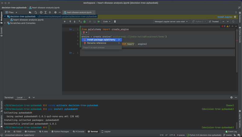
So how was this development experience different from working in JupyterLab? One of the first things I noticed is that all of the smart code completion and highlighting I’m used to from PyCharm is enabled within the DataSpell notebooks, which is an amazing upgrade from using regular notebooks or even JupyterLab. One of the first things I started benefitting from is the error detection. For example, you can see in the script below that when I tried to import a dependency I hadn’t installed yet, DataSpell threw an error.
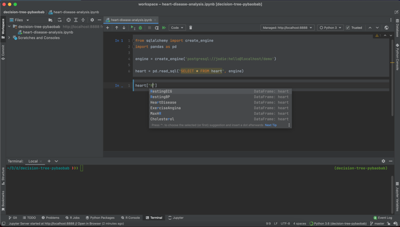
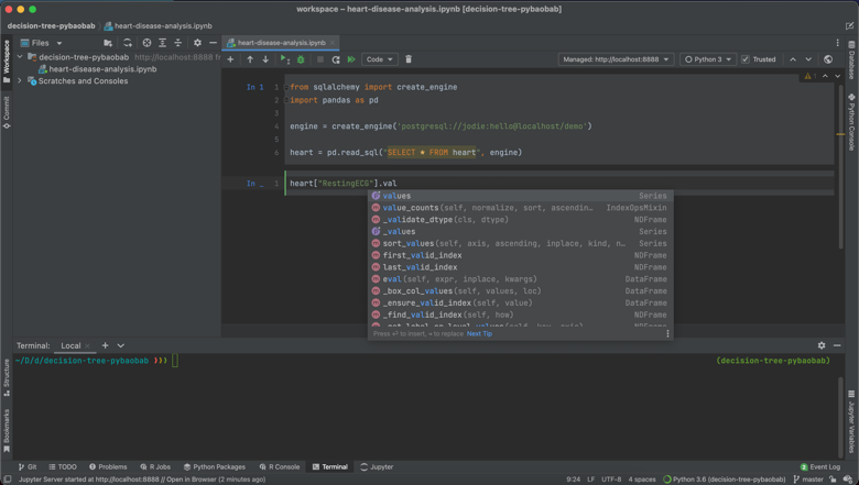
Secondly, I really like how nuanced the code completion is. As you can see in the following screenshots, the code completion is sensitive to context, suggesting methods, dataset names and column names in the correct places.
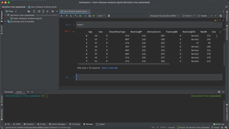
One final thing I really like is how Pandas DataFrames are displayed. I was able to view my complete DataFrame both within the notebook, and also have the option of opening it in a new tab, which really made scanning my data at the beginning of the project much easier. I imagine there are upper limits on the amount of columns and rows that you can display, but for smaller DataFrames, this is a lovely feature.
Visualising the decision tree
I’ll now use the pybaobab package to display an interpretable version of the decision tree model. As you can see, the labelling I did earlier of the target has appeared at the top of the chart, letting us know which branch belongs to which outcome. I’ve also customised it by using the standard Brewer colour themes, all of which are supported by pybaobab.
ax = pybaobabdt.drawTree(dt_class, size=15, dpi=150, features=features, colormap="PiYG")
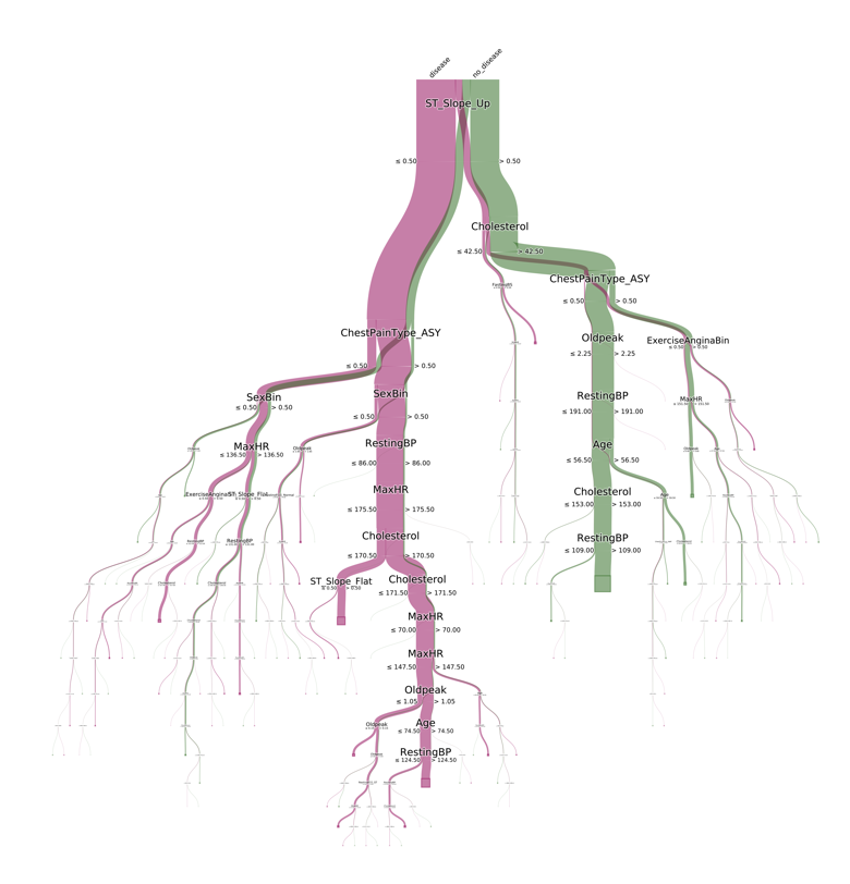
You can see that the main predictor of heart disease is people who don’t have an increasing peak ST segment while exercising. If we follow the pink line on this graph downwards, this traces the indicators in the model of having heart disease, including having asymptomatic chest pain, being female, and having a resting blood pressure of less than or equal to 86. While I’m not really able to interpret this model from a medical perspective, it’s easy to imagine such a visualisation being very useful for a cardiologist.
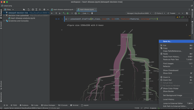
This visualisation actually came out very nicely in DataSpell. As you can see, I have my IDE set to a dark theme, and the visualisation is automatically displayed with a transparent background and white text. One other nice feature is that rather than having to explicitly save the visualisation with the savefig command, you can shortcut this by right clicking on the figure and saving it to file.
Splitting Python scripts
As you can see from the above, the notebook experience in DataSpell is very nice, but what about working with Python scripts? Let’s say that I want to be able to productionise this code, and I need to be able to run it in a Python script. My usual workflow for this is a little painful: normally I either do all of my prototyping in a Jupyter notebook and then export this to a .py file, or I start directly within a Python file, but comment out all of the code I don’t want to run as I test which parts are working.
The way that Python scripts are treated in DataSpell overcomes these issues. The first nice feature is that Python files can be split using the #%% separator, so that sections of the script are treated akin to the cells in Jupyter notebooks. This means you can run just one small section of the code at a time, just as you would with cells in the notebook. Secondly, the output of Python scripts can be written to an iPython console. Finally, you can view all of the Jupyter environment variables that have been created. You can see examples of this below for the data cleaning and model building components of the project we just completed.
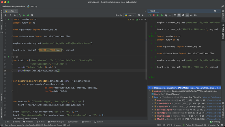
At the same time, the scripts still have the smart code completion, debugging and other development tools that come with PyCharm. This means you can get the best of both worlds: the editor supports you to break down the script, inspect the output and explore the data and models while you’re in the research phase of your project, but then allows you to switch to improving the code and getting it ready for production once the modelling is complete.
I’m only getting started with DataSpell and I am sure I have only scratched the surface of the available features, but so far I’ve really enjoyed the experience. I will keep exploring and report back with more cool features as I find them!
