Optimising the Minkowski distance, part 2: broadcasting
In the last blog post, we managed to shave a bit of time off our calculation of the Minkowski distance by using vector subtraction. Instead of calculating the difference between each pair of vectors elementwise using a loop, we were able to take advantage of NumPy’s vectorised implementation to take these differences in one pass.
However, we only knocked a couple of minutes off the calculation of the Minkowski distance on our second sample, which contained only three features but more than 13,000 observations. The main culprit of these long processing times is a remaining nested for loop which calculates the pairwise Minkowski distance between all observations in our samples. As such, we’ll be looking at how to use a method called broadcasting in NumPy to get rid of this and save ourselves some more time. Broadcasting is very powerful, but it’s not the most intuitive concept to understand. As such, we’ll be taking it slowly and explaining how we can apply it to our calculations step-by-step in this blog post.
Broadcasting
To understand how broadcasting works, let’s start with a small example. We’ll go back to the three example vectors we’ve been working with, \(X\), \(Y\) and \(Z\).
import numpy as np

X = np.array([5, 7, 3, 9])
Y = np.array([1, 6, 2, 4])
Z = np.array([8, 8, 3, 1])
In order to calculate the pairwise distance between each of these vectors, we’ll first combine all of them into a matrix with 3 rows and 4 columns. You can have a look at my earlier blog post for a fuller explanation of what a matrix is, but essentially it is just a table whose rows or columns are made up of a collection of vectors with the same number of elements. You can see the matrix we made below where \(X\), \(Y\) and \(Z\) make up the rows of the matrix.
print(np.array([X, Y, Z]))
[[5 7 3 9]
 [1 6 2 4]
 [8 8 3 1]]
In order to get the difference between each of the vectors and the \(X\) vector, we can create a second 3 x 4 matrix which is just composed of the \(X\) vector repeated three times:
print(np.array([X, X, X]))
[[5 7 3 9]
 [5 7 3 9]
 [5 7 3 9]]
We then subtract this matrix with the repeated \(X\) vector from the matrix containing all three vectors:
print(np.array([X, Y, Z]) - np.array([X, X, X]))
[[ 0  0  0  0]
 [-4 -1 -1 -5]
 [ 3  1  0 -8]]
We now have the pairwise differences between the elements of vector \(X\) and all other vectors, including itself. The reason this works is that the rules of vector subtraction also apply to matrices (see this blog post for an overview of this). Just as two vectors with the same number of elements can be subtracted from each other elementwise, we can also subtract two matrices of the same size from each other elementwise. In this case it’s possible as both of our matrices are 3 x 4. This looks like the following:

So far, so good. However, we still have one issue: if we want to also subtract vectors \(Y\) and \(Z\), we’re still stuck with a for loop, right? Well, there is a way to avoid this. At the moment, we are using 2-dimensional NumPy arrays, where the first dimension represents our number of vectors and the second dimension represents the number of elements in each vector.
np.array([X, Y, Z]).shape
(3, 4)
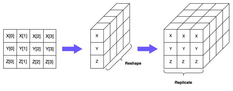
We can switch instead to using 3-dimensional NumPy arrays, where the first two dimensions represent the number of vectors, and the final dimension represents the number of elements in each vector. Let’s have a look at how this would work for the first array in our subtraction calculation:

In the second step in the above diagram, we’ve reshaped the 2-dimensional array containing \(X\), \(Y\) and \(Z\) into a 3-dimensional array with the dimensions \((1, 3, 4)\). This indicates we have three vectors (and only one copy of each of these) and each vector contains 4 elements.
np.array([[X, Y, Z]]).shape
(1, 3, 4)
In the final step in the diagram, we’ve just duplicated our reshaped matrix 3 times. As you can see, the dimensions of this array are now \((3, 3, 4)\), with the first dimension indicating that we have three copies of our original matrix.
np.array([[X, Y, Z], [X, Y, Z], [X, Y, Z]]).shape
(3, 3, 4)
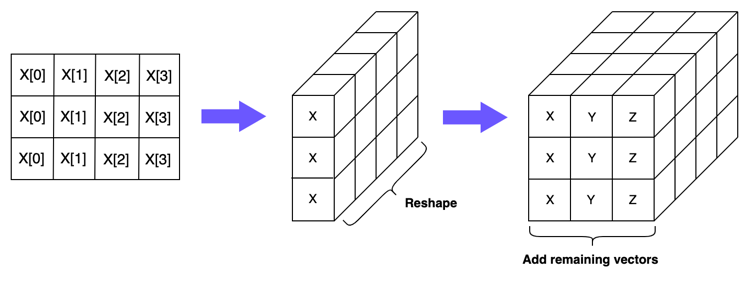
Now we need to create a corresponding array which will generate pairwise combinations of every vector when we do our subtraction. If you’ll recall, when we were working with the 2-dimensional arrays, we simply created a matrix which duplicated the vector \(X\) three times. We can do something similar here: we create 2-dimensional arrays which duplicate the \(Y\) and \(Z\) vectors three times. We can then reshape these matrices so that they are, again, of dimension \((1, 3, 4)\), and “stack” them within the same 3-dimensional array to get an array with dimensions \((3, 3, 4)\). Let’s see how this looks below:

Applying this in NumPy, you can see we do indeed get the correct shape:
np.array([[X, X, X], [Y, Y, Y], [Z, Z, Z]]).shape
(3, 3, 4)
Finally, if we subtract our new 3-dimensional arrays from each other, we’ll get the difference scores. When you see it in the diagram below, it’s pretty clear that we’ve successfully created the correct combinations of pairs:

Let’s check that it worked:
np.array([[X, Y, Z], [X, Y, Z], [X, Y, Z]]) - np.array([[X, X, X], [Y, Y, Y], [Z, Z, Z]])
array([[[ 0,  0,  0,  0],
        [-4, -1, -1, -5],
        [ 3,  1,  0, -8]],

       [[ 4,  1,  1,  5],
        [ 0,  0,  0,  0],
        [ 7,  2,  1, -3]],

       [[-3, -1,  0,  8],
        [-7, -2, -1,  3],
        [ 0,  0,  0,  0]]])
Great! We’re getting the numbers we expected.
However, it might have occurred to you that replicating each vector is not the most memory-friendly way of calculating the difference scores, especially once we start working with our full beans dataset or something even bigger. This is where broadcasting comes in. Essentially what broadcasting does is that it takes these replications that we’re doing explictly and implementing them in memory-efficient ways under the hood. Let’s have a closer look at how it works.
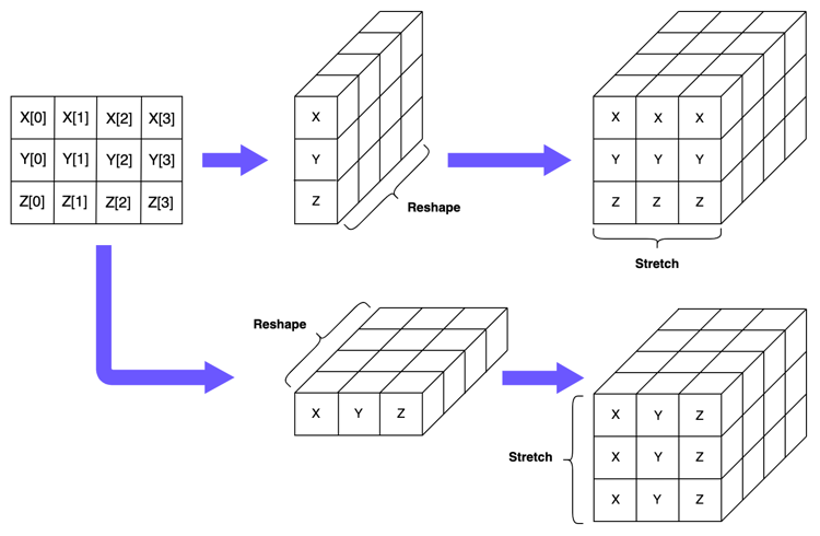
In order to get the correct pairwise subtractions earlier, we created a 3-dimensional array where our vectors were replicated across the columns in one array and across the rows in the second one. What we want to do with broadcasting is signal to NumPy that we want it to do the same thing for us. We do this by reshaping our 2-dimensional array into two 3-dimensional arrays, each “orientated” in different directions. In the first, we have the vectors sitting in the second dimension of the array, so that we end up with a \((1, 3, 4)\) array. In the second, we have the vectors sitting in the first dimension of the array, so that we end up with a \((3, 1, 4)\) array. NumPy will see the dimension where the size is 1 and realise it needs to “stretch” or duplicate the data along this dimension in order to make the arrays a compatible size for subtraction. Once it does this, the final output will be our \((3, 3, 4)\) array containing the difference scores.

Let’s have a look at this with our example vectors. We’ll first create our \((1, 3, 4)\) reshape of the 2-dimensional array:
np.array([[X, Y, Z]]).shape
(1, 3, 4)
We’ll then reshape it to a \((3, 1, 4)\) array:
np.array([[X], [Y], [Z]]).shape
(3, 1, 4)
Finally, we’re ready to do our subtraction:
np.array([[X, Y, Z]]) - np.array([[X], [Y], [Z]])
array([[[ 0,  0,  0,  0],
        [-4, -1, -1, -5],
        [ 3,  1,  0, -8]],

       [[ 4,  1,  1,  5],
        [ 0,  0,  0,  0],
        [ 7,  2,  1, -3]],

       [[-3, -1,  0,  8],
        [-7, -2, -1,  3],
        [ 0,  0,  0,  0]]])
And you can see we get the same results as when explicitly replicating the vectors! There is a slightly nicer notation for reshaping our arrays which I will use going forward. We can take advantage of the fact that when we pass None to slicing operations in NumPy, NumPy will automatically assign a dimension of 1 (as there is no data in that dimension).
np.array([X, Y, Z])[None, :, :].shape
(1, 3, 4)
np.array([X, Y, Z])[:, None, :].shape
(3, 1, 4)
np.array([X, Y, Z])[None, :, :] - np.array([X, Y, Z])[:, None, :]
array([[[ 0,  0,  0,  0],
        [-4, -1, -1, -5],
        [ 3,  1,  0, -8]],

       [[ 4,  1,  1,  5],
        [ 0,  0,  0,  0],
        [ 7,  2,  1, -3]],

       [[-3, -1,  0,  8],
        [-7, -2, -1,  3],
        [ 0,  0,  0,  0]]])
You can see it gets us the exact same result as when using the bracketing notation, and is much easier to read (especially for larger arrays).
Now that we understand broadcasting, we can overhaul our Minkowski distance functions to use it, rather than that inefficient nested for loop. You can see that instead of calculating the difference between one pair of vectors, the formula now takes in two matrices (such as the bean dataset) and calculates the pairwise difference between all rows.
def calculate_minkowski_distance_vectorised(array1: np.ndarray,
                                            array2: np.ndarray,
                                            p: int
                                            ) -> np.ndarray:
    """
    Generalised formula for calculating both Manhattan and Euclidean distances. Calculates pairwise distances between every point in two n-dimensional arrays.
    array1: first set of points;
    array2: second set of points;
    p: power parameter which determines the distance metric used, with 1 = Manhattan and 2 = Euclidean.
    """

    diffs = array1[:, None, :] - array2[None, :, :]
    abs_diffs = np.power(np.abs(diffs), p)
    return abs_diffs.sum(axis=-1) ** (1 / p)
Let’s test it out.
%time vect_min_1 = calculate_minkowski_distance_vectorised(array_sample_1, array_sample_1, 2)
CPU times: user 1.48 ms, sys: 947 µs, total: 2.42 ms
Wall time: 1.2 ms
%time vect_min_2 = calculate_minkowski_distance_vectorised(array_sample_2, array_sample_2, 2)
CPU times: user 13.3 s, sys: 3.23 s, total: 16.5 s
Wall time: 16.6 s
%time vect_min_3 = calculate_minkowski_distance_vectorised(array_sample_3, array_sample_3, 2)
CPU times: user 1min 30s, sys: 1min 48s, total: 3min 18s
Wall time: 5min 38s
We’ve now been able to lower our calculation time for 3 features and ~13,000 observations to less than 20 seconds, which is an incredible improvement over the 13 minutes we saw when using the nested for loops. However, with 16 features our performance is still a bit slow. Fortunately, we still have a couple more tricks we can use, which we’ll cover in the next blog post.
